What resolution should my microscope's digital camera have?

Original source: http://www.microscopiaoberta.com/?p=184&lang=ca

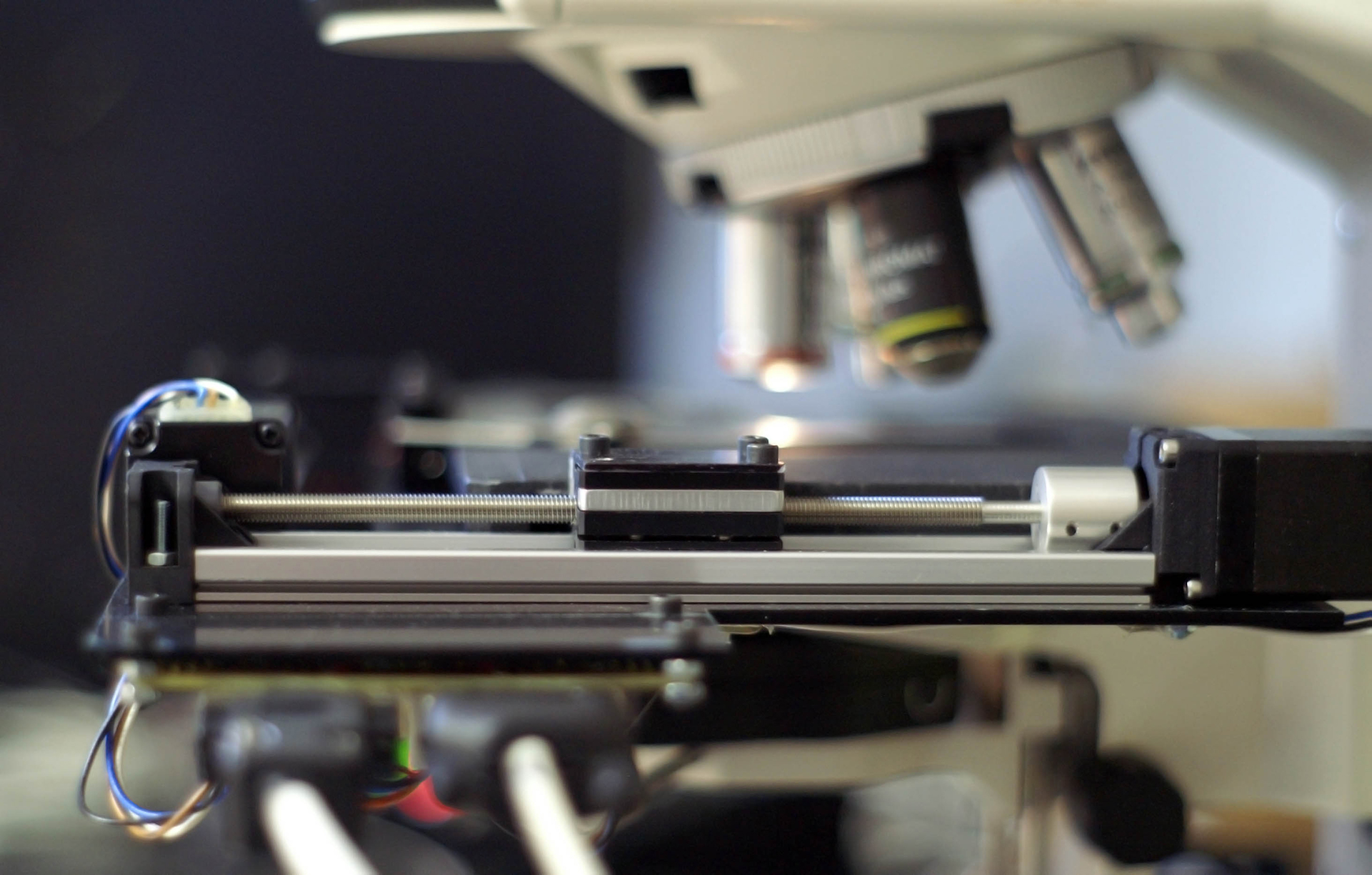
It’s a classic for customers to ask me about digital cameras with ‘the more megapixels, the better.’ However, I always respond the same when they ask me this question:

The separating power (A.K.A. resolution) of a microscope is not given by the camera, is given by the objective of the microscope.

However, in the market, there are microscope cameras ranging from 1 to 32 megapixels, with 5 and 10 megapixels being common. But if the resolving power/resolution is not provided by the camera…

How many pixels are needed to work with microscopy?

Well, here I will present my proposal of mathematical demonstration, being as ‘objective’ as possible.

First point – The resolving power (A.K.A. Resolution) of a microscope

To determine HOW MANY pixels we need, we first need to know the resolving power of our microscopes.

This parameter is mainly determined by the Numerical Aperture of our objectives and is defined by the following simplified formula :

Form 1 Resolving Power [1]

Editor’s note (2026): 0.61·λ/NA is the Rayleigh criterion (two incoherent points, ~26% intensity dip) — the correct, practical criterion for a camera. It differs from the Abbe diffraction limit d = λ/(2·NA) (the information limit, based on capturing the first diffracted order) by a factor of 1.22 (the first zero of J₁/π). The theoretical information limit is therefore about 20% finer than the Rayleigh value used here.

Where:

Table Resolving Power µm

Second point – Nyquist’s Theorem

Now we have the resolution of our objectives, but how does this translate into pixels?

Well, for this, we have Nyquist’s Theorem [2], which will determine the IDEAL pixel size for each of our objectives. I won’t go into depth on the theorem; for more information, consult Wikipedia .

A formula to calculate the IDEAL pixel size in microscopy is:

Form 2 Pixel Ideal Size µm [3]

Editor’s note (2026): Nyquist’s theorem strictly applies to the optical cut-off frequency f_c = 2·NA/λ (incoherent illumination), not to the Rayleigh criterion. Strict Nyquist requires p ≤ M·λ/(4·NA); the formula used above (p = 0.61·λ·M/(2·NA)) is 1.22× more relaxed — a conservative engineering rule (it matches the Nikon MicroscopyU pixel calculator, ref. [3]), not the theorem itself. It never recommends under-sampling. Also, meeting Nyquist guarantees information can be transferred, not that it is fully usable: near f_N the optical MTF has already dropped, and a square pixel’s own MTF is sinc(p·f) = 0.637 at its own Nyquist frequency. In practice, 2.5–3 pixels per resolved element is a safer target than 2.

M	NA	p ideal, article (µm)	p Nyquist strict (µm)	ratio
10	0.25	6.77	5.55	1.22
20	0.40	8.46	6.94	1.22
40	0.65	10.42	8.54	1.22
63	0.85	12.55	10.28	1.22
100	1.25	13.54	11.10	1.22

Where:

Now we add a column to our Resolving Power table with the Ideal Pixel column in µm:

Table Dimensions Pixel Size Ideal µm [3]

Third point – Camera Sensor Size

Now we know what dimensions our pixels need to have to resolve the images from our microscopes in maximum detail… but (there’s always a ‘but’) how do we translate the size of 1 pixel into the resolutions we use with our cameras?

The simplest way to calculate is:

Form 3 Dimension Pixel Ideal

Where we consider that pixels are SQUARE.

For a theoretical sensor with a 1-inch diagonal and a 4/3 aspect ratio, we obtain:

Table Maximum Megapixels For each magnification

⚠ Correction (added 2026): the tables below treat "1 inch" as a literal 25.4 mm diagonal. Sensor-format designations (1", 1/2", 1/3"…) are historical optical labels inherited from vidicon tubes — not physical measurements:

Format	Literal diagonal (used in this article)	Real dimensions
1"	25.4 mm	12.8 × 9.6 mm (diagonal ≈ 16 mm)
1/2"	12.7 mm	6.4 × 4.8 mm
1/3"	8.47 mm	4.8 × 3.6 mm
1/2.5"	10.16 mm	5.76 × 4.32 mm

As a result, every "maximum megapixels" table in this article is inflated by roughly 2–2.5×. With real sensor dimensions, a 1/3" sensor at M=10 supports about 0.56 MP, not the much larger figure implied by a literal 25.4 mm diagonal — modern 1/3" microscopy sensors (2–4 µm pixels) intentionally oversample relative to the "ideal pixel" computed here. Always use the real physical dimensions of your specific camera sensor model, not the inch label, when sizing a camera.

Corrected table — maximum megapixels with strict Nyquist (p = M·λ/(4·NA)), real sensor dimensions
M	NA	p Nyquist (µm)	1/3" real (4.8×3.6)	1/2" real (6.4×4.8)	1" real (12.8×9.6)
10	0.25	5.55	0.56 MP	1.00 MP	3.99 MP
20	0.40	6.94	0.36 MP	0.64 MP	2.55 MP
40	0.65	8.54	0.24 MP	0.42 MP	1.69 MP
63	0.85	10.28	0.16 MP	0.29 MP	1.16 MP
100	1.25	11.10	0.14 MP	0.25 MP	1.00 MP

Above the MegaPixels value obtained, we will be oversampling the image and NOT OBTAINING MORE INFORMATION, just bigger/larger spots with more pixels but not more ‘resolved’ images/information.

Below this value, we do LOSE INFORMATION, and it is not recommended at all (if we can avoid it, of course!).

Editor’s note (2026): oversampling does not lose information, and it is not purely wasteful — it gains sampling robustness, keeps frequencies closer to the optical cut-off, and improves Bayer demosaicing quality. Modern microscopy sensors oversample deliberately. What oversampling costs is per-pixel signal-to-noise ratio and file size, not resolution. A practical target is a pixel size between the strict Nyquist value and about 1.5× that value — "fewer megapixels" is not a strict requirement.

An important detail to consider here is that our sensor doesn’t have ANY additional optical element that could modify the dimensions of the sensor.

In the case that our microscope has a 0.63x or 0.5x adapter for the camera, we will need to recalculate the sensor size with the following formula:

Form 4 RealSensorSize/Magnificaion Adapter camera

Example of a 1/3″ with a 0.5x optical camera adapter:

Let’s compare the results of the maximum MegaPixels with and without the optical camera adapter:

Table: Maximum Megapixels for a 1/3″ Sensor Camera with 1x adapter:

Table: Maximum Megapixels for a 1/3″ Sensor Camera with 0.5x adapter

Here we see the dual utility of optical adapters for cameras in microscopes because, in addition to increasing the ‘field’ of our image, they also allow us to obtain images at higher ‘megapixels,’ at the cost of losing magnification, of course!

Notes:

This Ideal Pixel dimension and all the tables presented so far correspond to a MONOCHROME sensor.

RGB camera sensors, which usually have a color filter with a Bayer pattern, the usable pixel does NOT correspond to the pixel size provided by the manufacturer because it is necessary to apply DeMosaicing [4] (color interpolation) to obtain a pixel with the correct RGB color, altering the effective pixel size according to the DeMosaicing method/algorithm applied, with typical factors between 1.25x and 2x depending on the method used.

Only monochrome sensors meet the nominal Nyquist pixel size computed above. For RGB/Bayer sensors, multiply the strict Nyquist pixel size by the demosaicing factor (p_Bayer ≈ 2 × p_Nyquist for standard bicubic interpolation).

Further technical notes (2026):

The full system MTF is a product: MTF_system = MTF_optics × sinc(p·f) × fill factor — this is the framework that explains why the "ideal pixel" is not an all-or-nothing threshold.
This criterion assumes well-adjusted Köhler illumination (condenser NA ≥ objective NA); with a closed condenser, coherence increases and the cut-off shifts to NA/λ (coherent illumination).

Thanks for your attention

F.Xavier Gómez

References

[1] https://en.wikipedia.org/wiki/Optical_resolution

[2] https://en.wikipedia.org/wiki/Nyquist-Shannon_sampling_theorem

[3] http://www.microscopyu.com/tutorials/java/digitalimaging/pixelcalculator/

[4] https://en.wikipedia.org/wiki/Demosaicing

All information published here is under the license Creative Commons Attribution-NonCommercial 4.0 International License.